
The beginner's guide to implementing simple linear regression using Python
In this post, we will be putting into practice what we learned in the introductory linear regression article. Using Python, we will construct a basic regression model to make predictions on house prices.

Introduction
Linear regression is a type of analysis used to make predictions based on known information and a single independent variable. In the previous post, we discussed predicting house prices (dependent variable) given a single independent variable, its square footage (sqft).
We are going to see how to build a regression model using Python, pandas, and scikit-learn. Let's kick this off by setting up our environment.
Setting up your system
Installing Python
Let's start by installing Python from the official repository: https://www.python.org/downloads/
Download the package that is compatible with your operating system, and proceed with the installation. To make sure Python is correctly installed on your machine, type the following command into your terminal:
python --versionYou should get an output similar to this: Python 3.9.6
Installing Jupyter Notebook
After making sure Python is installed on your machine (see above), we can proceed by using pip to install Jupyter Notebook.
In your terminal type the following:
pip install jupyterOnce installation is complete, launch Jupyter Notebook in your project directory by typing the following:
jupyter notebook
This command will automatically open your default browser, and redirect you to the Jupyter Notebook Home Page. You can select or create a notebook from this screen.
Creating a new Jupyter Notebook
For this exercise, we'll create a new notebook by clicking on New -> Python3 as shown below:
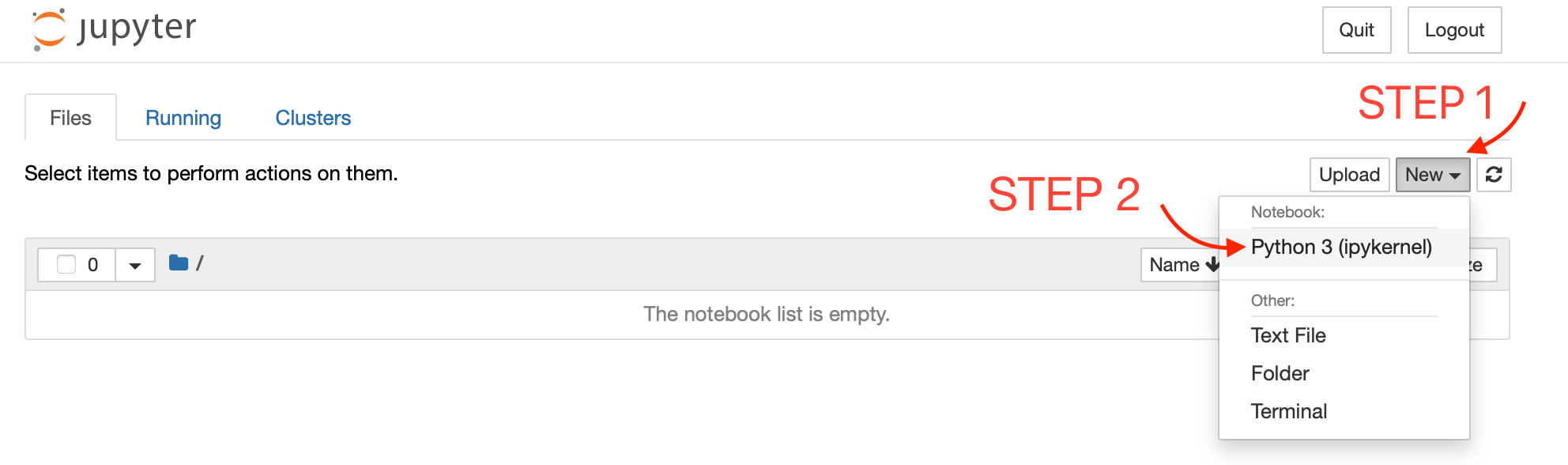
Great! That's it. We're all set up and ready to get started.
Data Collection
We'll start by importing pandas. This is a Python library that makes it easy for us to manipulate and analyze data. To import the library, we will use the following:
import pandas as pdNext, we'll create our dataset as a pandas DataFrame. Think of the DataFrame as an Excel or SQL table. We can manipulate and process data easily once it's in the pandas DataFrame type.
# Create the DataFrame
data = pd.DataFrame({
    'House': [1, 2, 3, 4, 5, 6, 7, 8, 9, 10, 11, 12, 13, 14, 15, 16, 17, 18, 19, 20],
    'SquareFootage': [1000, 1200, 1500, 1800, 2200, 1350, 2000, 1750, 1650, 1900, 1300, 2500, 1400, 2050, 2250, 1600, 1950, 2200, 1800, 1250],
    'Price': [100000, 150000, 200000, 250000, 300000, 175000, 225000, 210000, 195000, 240000, 160000, 325000, 170000, 235000, 275000, 190000, 230000, 300000, 250000, 145000]
})
We can use the .head() method of the DataFrame to display the first five rows of data, and the .describe() method to print a relevant statistical summary of the dataset.
Let's take a look at both methods:
# Print the first five rows of data
data.head()| SquareFootage | Price | |
|---|---|---|
| 0 | 1000 | 100000 |
| 1 | 1200 | 150000 |
| 2 | 1500 | 200000 |
| 3 | 1800 | 250000 |
| 4 | 2200 | 300000 |
# Get a statistical summary of DataFrame
data.describe()| SquareFootage | Price | |
|---|---|---|
| count | 20.000000 | 20.00000 |
| mean | 1732.500000 | 216250.00000 |
| std | 405.642765 | 58125.88426 |
| min | 1000.000000 | 100000.00000 |
| 25% | 1387.500000 | 173750.00000 |
| 50% | 1775.000000 | 217500.00000 |
| 75% | 2012.500000 | 250000.00000 |
| max | 2500.000000 | 325000.00000 |
Data Wrangling
For our project, and to keep things simple, I am just going to modify the data by dropping the 'House' column since it is irrelevant. To do that, we use the .drop method of the DataFrame:
# Drop the 'House' column
data = data.drop('House', axis=1)

# Perform other data wrangling operations if necessary...
I'm not going to do any further data manipulation. It's important to note, however, that Data Wrangling is a very important step in the process, specifically, you'll need it when dealing with missing values, outliers, scaling, normalization, feature engineering, and more.
Splitting the Data
To train our model, we'll need to split our dataset into two sets. Usually, the split is 80/20, meaning 80% of the data will be used for training and the remaining 20% for testing.
Luckily, sklearn's built-in train_test_split function helps us do just that. Using this method, we can set the training and testing variables, as seen here:
from sklearn.model_selection import train_test_split

# Split the data into training and testing sets
X = data['SquareFootage'].values.reshape(-1, 1)

# Independent variable
y = data['Price'].values  # Dependent variable

X_train, X_test, y_train, y_test = train_test_split(X, y, test_size=0.2, random_state=42)
X refers to our independent variables (all the square footage values), and y to our dependent variables (all the corresponding prices). The linear regression algorithm will use that data to learn and be able to make predictions.
train_test_split takes in X and y, test_size (The percentage of data to use for testing), and random_state (The seed value for the random number generator, the value itself does not matter but it is used to maintain consistent results when running the same code with the same value multiple times).
What the code above does, essentially, is split the dataset data into four variables:
- X_train and y_train: These variables will contain 80% of randomly chosen values from the dataset used for training.
- X_test and y_test: These variables will contain 20% of randomly chosen values from the dataset used for testing.
Fitting the Model
Easy so far? Should be, because we're almost done. Now since our training and testing variables are set, we can go ahead and fit the model.
from sklearn.linear_model import LinearRegression

# Create the regression model object
model = LinearRegression()

# Fit the model to the training data
model.fit(X_train, y_train).fit() method which basically does everything for us.To print the values of β₀ and β₁. We can use the .intercept_ and .coef_[0] properties of the model as such:
# Print the values of β₀ and β₁
print("Intercept (β₀):", model.intercept_)
print("Slope (β₁):", model.coef_[0])

# Intercept (β₀): -7623.808416647284
# Slope (β₁): 129.38851429900024
β₀ and β₁
Checking Model Accuracy
Great stuff. With the help of sklearn we found our intercept, and slope values by fitting a straight line into our scattered data points. We can quickly run an accuracy check by looking at the R-squared value on the testing set:
# Calculate R-squared on the testing set
r_squared = model.score(X_test, y_test)
print(f'R-squared: {r_squared:.2f}')

# R-squared: 0.95
An R-squared value of 0.95 is considered very good in the context of simple linear regression. The value is between 0 and 1, and the 0.95 value in our case indicates that 95% of the variation in the price, can be explained by the independent variable (square footage), which indicates a strong correlation.
Making Predictions
We're basically done. Now the moment of truth, we can use our newly trained model to make some house price predictions given one (or more) sqft values.
Let's try to predict the house price given a set of three houses that have areas of 1100, 1700, and 2000 sqft:
# Prediction time!
new_sqft = [[1100], [1700], [2000]]
predicted_prices = model.predict(new_sqft)

# Print the predicted prices
for sqft, price in zip(new_sqft, predicted_prices):
    print(f'sqft: {sqft[0]} => price: {price:.2f}')

# sqft: 1100 => price: 134703.56
# sqft: 1700 => price: 212336.67
# sqft: 2000 => price: 251153.22
Predicting house prices using .predict()
Conclusion
Congratulations on making it this far. We've seen how we can collect, modify, organize, and prepare to fit data into a linear regression model, calculate its accuracy, and make predictions! Python and its open-source libraries make it easy for us to do most of the math and optimizations as you've seen. Go ahead and experiment with your own dataset!