
An introduction to multiple linear regression for machine learning
In this post, we'll define what Multiple Linear Regression is, and its use cases, then we'll dive deep into the algorithm how it's applied, and the best practices.

A Brief Overview
Simple Linear Regression is used in Machine Learning and Statistics to predict an outcome (ŷ) given a single variable (x). For example, Simple Linear Regression is used to predict a house price, given its area size. In this post, we'll focus on the same exercise of predicting a house price given its area size (sqft).
Mulitple Linear Regression is used when we have more than a single independent variable. For our example, we're going to add a couple of extra variables other than the area size (sqft):
- New variable 1 (or x2): Number of bedrooms
- New variable 2 (or x3): Number of bathrooms
Keep in mind that x1 is our previous square footage (in sqft)
Here's the table from the previous article, modified to include the new independent variables (IVs), Bedrooms, and Bathrooms as shown below:
| House # | Square Footage (x1) | Bedrooms (x2) | Bathrooms (x3) | Price ($) |
|---|---|---|---|---|
| 1 | 1000 | 1 | 1 | 100000 |
| 2 | 1200 | 2 | 1 | 150000 |
| 3 | 1500 | 2 | 2 | 200000 |
| 4 | 1800 | 3 | 1 | 250000 |
| 5 | 2200 | 3 | 2 | 300000 |
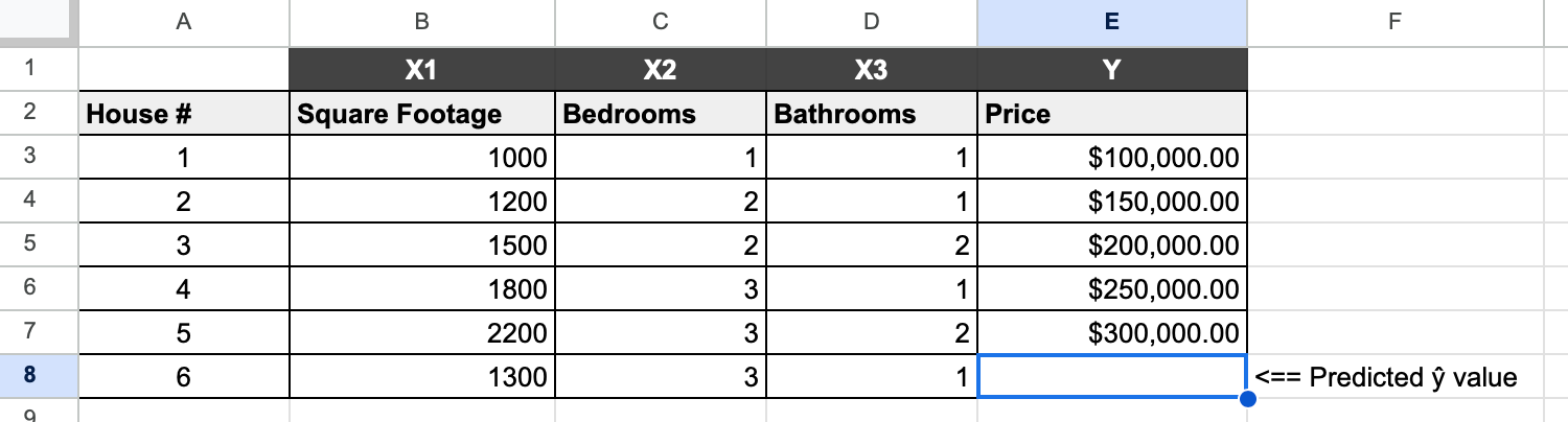
We'll go ahead and add a new house to the table. We know the following:
- It has an area of 1300 sqft
- It has 3 Bedrooms
- It has 1 Bathroom.
Here it is, added as a new row in our table:
| House # | Square Footage (x1) | Bedrooms (x2) | Bathrooms (x3) | Price ($) |
|---|---|---|---|---|
| ... | ||||
| 6 | 1300 | 3 | 1 | ?? |
Since we now have three variables, we'll use the Multiple Linear Regression equation to make our prediction:
$$ \hat y = b_0 + b_1 x_1 + b_2 x_2 + ... + b_k x_k $$
Which in our case translates to:
$$ \hat y = b_0 + b_1 x_1 + b_2 x_2 + b_3 x_3 $$
The coefficients are interpreted similarly to the Simple Linear Regression equation while taking into account the added variables (number of bedrooms, and bathrooms).
Complicated? Let's break it down:
- ŷ is our dependent variable (DV) = price in our case
- Our independent variables (IVs):
- x1 = 1300 (Square Footage)
- x2 = 3 (Bedrooms)
- x3 = 1 (Bathroom)
- b0 is the intercept
- It is the value of ŷ when all values of x = 0
- b1, 2, 3 are the coefficients, each will estimate the change in ŷ (predicted house price) for every 1 unit change in a variable when all other variables are constant.
The predictors, b1, b2, and b3 are calculated exactly like we've calculated b1 in our previous article, you can check it out here.
It's important to note that b0 is also similar, but takes into consideration the extra independent variables, so our b0 equation becomes:
$$ b_0 = \bar{y} - b_1\bar{x}_1 - b_2\bar{x}_2 - ... - b_p\bar{x}_p $$
Multiple Linear Regression Simulation
Here's a simple example showing the Multiple Linear Regression formula in action. Let's plug in the following test values and analyze their impact on the predicted price:
Let's assume that:
b0 = 30500
b1 = 90 (Square Footage predictor)
b2 = 4000 (Number of bedrooms predictor)
b3 = 1250 (Number of bathrooms predictor)
These values are just chosen randomly for the purpose of this example and do not apply in a real-world scenario.
Our equation looks like this:
$$ \hat y = 30500 + 90 x_1 + 4000 x_2 + 1250 x_3 $$
Similarly, we can see that the same logic applies here as we've seen for the Simple Linear Regression.
A single unit increase in the square footage (x1) will result in a 90$ (b1) increase in the house price. In our case, 90 (1300) = 117000$ increase for the 1300 sqft. This is given that all other independent variables (x2, x3) remain constant.
Based on the simulation above, and assuming all other variables are constant, what is the increase in house price if the house has 10 bathrooms?
Knowing that 4000 represents our bathroom coefficient which indicates the change in house price for each 1 bathroom increase, and we have 10 bathrooms, we can simply multiply 10 by 4000 to get a total of 40000$ increase in the total price.
Include or Exclude IVs?
How to decide which independent variables (IVs) to include and which to exclude? Well, there are some key considerations:
- Visualize your data by creating scatterplots using any visualization tool to determine which independent variables have a weak correlation with the dependent variable.
- Perform analysis using Microsoft Excel or Google Sheets (or any other tool/library). This can help in confirming your scatterplot observations.
Let's take a closer look at the above points.
Visualizing Data with Scatterplots
Price and house area (in sqft) relationship
Let's start by creating a scatterplot of the house area (in sqft) on the x-axis, and the price in dollars on the y-axis, as seen below:

It's clear that there is a strong correlation between the two variables since we can easily fit a straight line through the points. We can, therefore, note that the square footage (sqft) is a strong candidate for inclusion in our regression equation. Let's take another example and visualize the relationship between the price and the number of bathrooms.
Price and number of bathrooms relationship
Let's take a look at the scatterplot with the number of bathrooms variable on the x-axis, and the house price on the y-axis:

As we can see from the chart above, our third independent variable, in this case, the number of bathrooms does not have a strong or any linear relationship with our dependent variable, price. Based on this observation, the number of bathrooms might not be a strong candidate to include in our regression equation.
You can perform the last visualization yourself to determine the correlation between the number of bedrooms and price.
Checking for Multicollinearity
Now let's check the correlation between our independent variables individually (excluding the dependent variable: price) to check for multicollinearity.
In statistics, multicollinearity is a phenomenon in which one predictor variable in a multiple regression model can be linearly predicted from the others with a substantial degree of accuracy.
Simply put, multicollinearity is when we have two or more independent variables that are highly correlated with each other. For example, if we want to predict how fast a car can go, and we include both the weight and the size of the car as predictor variables, we might have a problem because these variables are closely related. This can make it difficult to interpret the effects of each variable on the car's speed. In that case, we'll want to exclude one of the variables from our final equation.
Let's observe the scatterplot showing the area of the house (sqft) on the x-axis, and the number of bedrooms on the y-axis:

This can be done for each of the independent variables, but I've taken this example to show that we can detect a significant relationship between these two independent variables, where we can easily fit a straight line through the data points. If you take a look at the R2 value at the top of the scatterplot, you'll see that it's 0.772. This indicates that there is a strong correlation between square footage and number of bedrooms.
Since we're looking at the correlation between two independent variables, the data above tells us that there is a high correlation between square footage and number of bedrooms. This indicates that we should consider excluding one or both of them from our regression equation.
Based on the above, we should have an idea which independent variable(s) we could consider excluding from our regression formula.
Correlation Analysis
Correlation Coefficient r using =CORREL(...)
Let's compute the correlation coefficient (also known as Pearson r or Pearson correlation coefficient). We do this by using the CORREL(...) function built into Microsoft Excel or Google Sheets.
Here are the results for all the variables:
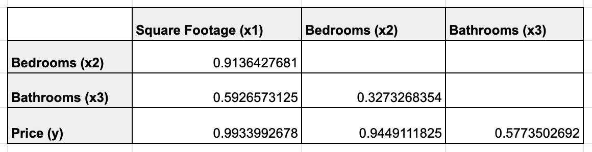
This further reinforces our initial observation that the relationship between square footage and the number of bedrooms is strong (0.9136427681 or ~91%), an indication of multicollinearity (Since this is a relationship between two independent variables). It also confirms our observation that the relationship between the number of bathrooms and price is not so strong ~58%.
You do not need to perform all of the above manually since modern libraries and statistical software can automatically tell us which variables to exclude from our model. But, you now have a good understanding of how the software is generating its recommendations.
Basically, it will look at all the possibilities, from which it will select the equation having the least complexity while taking out the variables causing multicollinearity and/or having a weak correlation with the dependent variable.
Bringing Everything Together
While you can do the math manually yourself to generate a prediction, there are obviously faster ways. For this example, we'll use Google Sheets and XLMiner Analysis ToolPak.
First, we fill in our existing data as shown below:
Then we'll use the XLMiner Add-on to generate our multiple linear regression summary analysis as shown below:
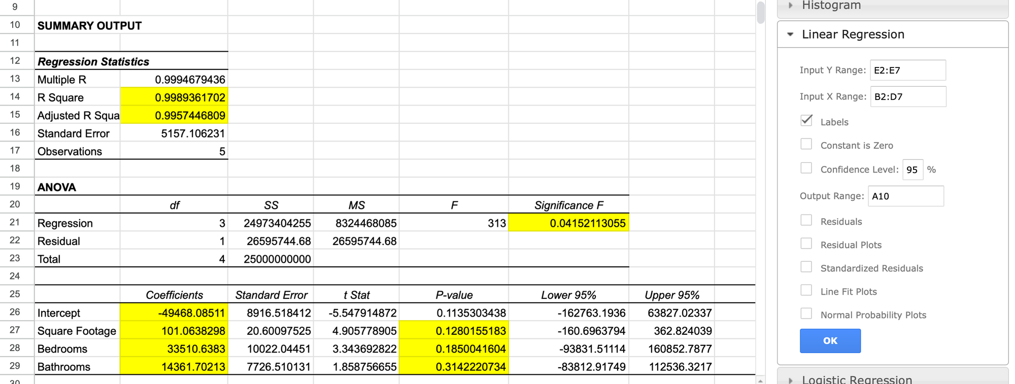
There we have it, everything is computed for us and we have everything we need to build our multiple linear regression equation. I've highlighted the Coefficients for each of our independent variables and our intercept b0 as seen on rows 26 to 29.
Using the values above, let's replace:
$$ \hat y = -49468 + 101 (x_1) + 33511 (x_2) + 14362 (x_3) $$
$$ \hat y = -49468 + 101 (1300) + 33511 (3) + 14362 (1) = $196,808.51 $$
And that's it, our predicted house price is $196,808.51. We can test the equation using values of any house from #1 to #5 from our table to see if our predictions are accurate. To demo this, I've computed the values of house #1 to compare the prediction with the actual price:
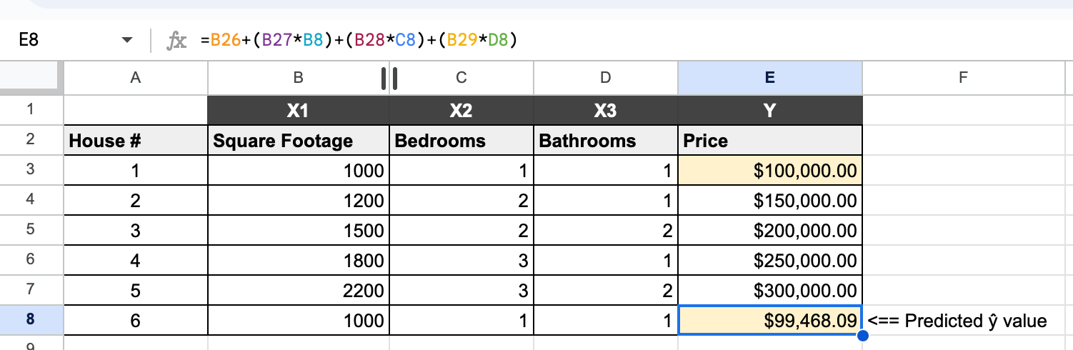
As you can see, our predicted value of $99,468 is very close to the known house price of $100,000 in row 1. This indicates that our model has a high accuracy. In machine learning, our model will use a test set to predict a dependent variable and then the results will be compared with the actual values from our data set to determine accuracy. We'll cover how a decrease in prediction errors and accuracy improvement is done in Machine Learning in a separate post, so stay tuned for more!
Conclusion
In the real world, you'll most likely deal with multiple independent variables. Given what we've seen so far, you'll know what goes on behind the scenes when you're using a Python library or another tool to set up regression-based models.
Thanks for reading!