
Here's how you can implement Gradient Descent using JavaScript
In this post, we're going to see how online gradient descent is implemented with JavaScript to determine the best parameters for a simple linear regression model to make accurate predictions.

Introduction to Gradient Descent
Gradient Descent or Online Gradient Descent is a widely used optimization algorithm in Machine Learning and Deep Learning. The purpose of Gradient Descent is to train a model iteratively to determine its optimal predictie values (weight, and bias) by minimizing its cost function.
Imagine you're about to skydive, and your goal is to land at the base of a valley. You're carrying with you a special sensor that tells you whether the ground is getting steeper or flatter as you descend. You'll be using this sensor to adjust your movements and direction so you can reach the bottom of the valley as quickly as possible.
We'll call the movements you make "parameters", and the special sensor "gradient". As soon as you jump from the plane you start descending, based on the special sensor feedback (aka gradient), you optimize your movements to move in the direction leading to the quickest descent. This iterative process of using the gradient to guide your movements ensures that you are constantly moving in the optimal trajectory. Finally, we'll call the distance between the initial location to the bottom of the valley the "cost (or loss) function".
Here's a beautiful drawing that I made to illustrate this example:
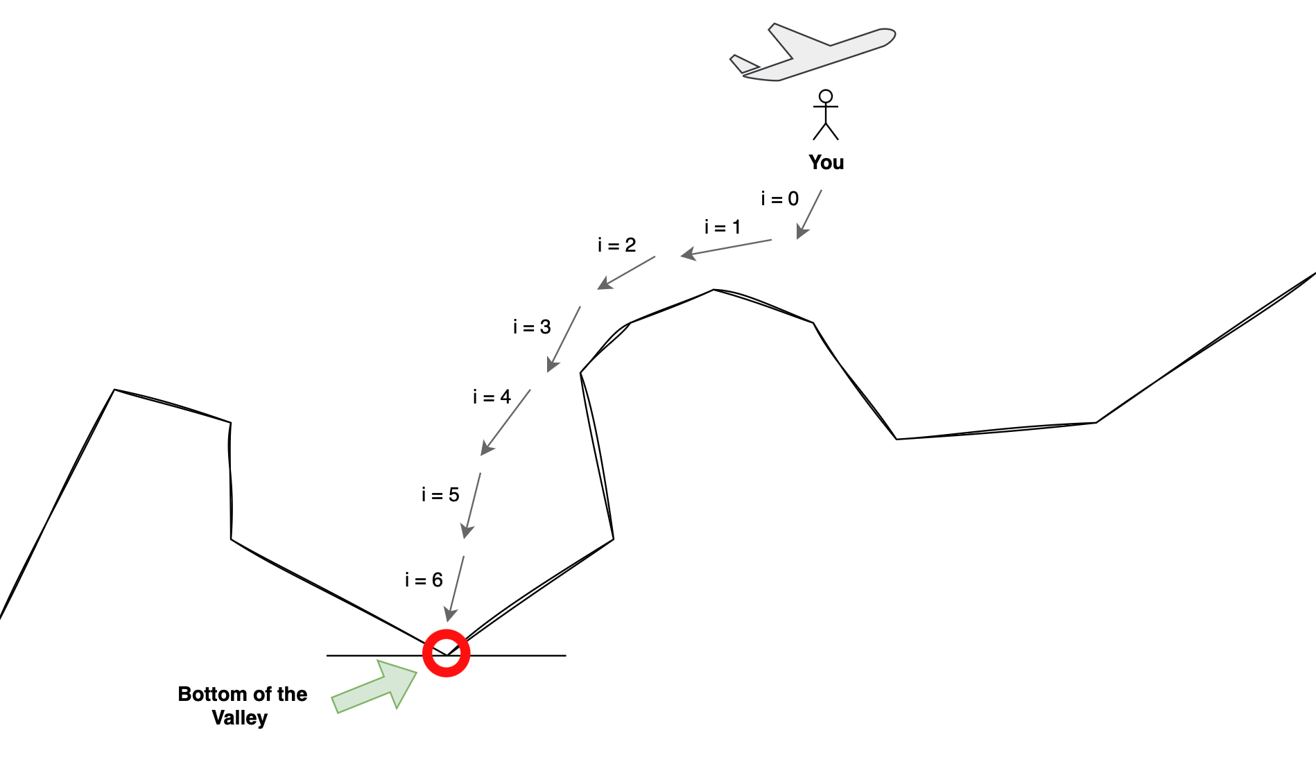
With that in mind and. as you can see, the skydiver made 7 movement adjustments to reach the bottom of the valley from the starting point. At each step, the skydiver used their current position to determine the next best movement. They did this by feeding the current position into the special sensor, which it used to compute the best next position adjustment. This process continued until the skydiver safely arrived at the bottom of the valley.
Some keywords from what we've seen so far:
- Gradient = Special Sensor
- Parameters = Movements (or Positions)
- Cost = Distance from starting point to the bottom of the valley
Use Cases
Now that we understand what gradient descent is in theory, and what it's used for, let's explore some real-world machine learning problems including corresponding cost functions that can be minimized using gradient descent:
| Use Cases | Cost Functions | Details |
|---|---|---|
| Linear Regression | Mean Squared Error (MSE) | Predicting housing prices based on features |
| Logistic Regression | Cross Entropy Loss | Classifying emails as spam or non-spam |
| Neural Networks | Cross Entropy Loss | Image recognition for identifying objects or faces |
| Support Vector Machines (SVM) | Hinge Loss | Classifying emails as spam or non-spam |
| Recommender Systems | Mean Squared Error (MSE) | Recommending movies or products to users |
These are a few examples of the many applications of gradient descent in the real world.
Next, we're going to explore how gradient descent is used to minimize the cost function Mean Square Error (MSE) of a linear regression problem that will predict house prices based on a single feature, the area size.
Implementing Gradient Descent for Simple Linear Regression Model in JavaScript
For this example, let's assume we have a training set consisting of the below JavaScript arrays X_values and y_values where X_values represent the area sizes (in 100 sqft), and y_values represent the corresponding prices (in thousands of dollars), as such:
var X_values = [1, 2, 3, 4];
var y_values = [200, 300, 450, 700];
Training Data X_values and y_values
1 * 100 = 100, and the price is 200 * 1000 = 200000. Then the second house has an area of 200 sqft and a price of 300K, and so on...Simple Linear Regression
The simple linear regression equation is:
$$f_{w,b} = wx + b$$
This equation takes in w which is known as the coefficient (or weight), and b which refers to the intercept (or bias). x is our known parameter, in our case, x is a new house area size, and $f_{w,b}$ or simply y is the predicted house price.
We can make predictions using the above equation by computing $f_{w,b}$ given w and b.
You might be asking:
- We know what
xis, but how do we choose the values ofwandb? - Then, how do we adjust the values of
wandbuntil optimal values are found?
Choosing w and b
A common practice in Machine Learning is to start off with w and b set to 0 (zero). This is because it simplifies implementation and is a good starting point for the optimization process.
w and b are also commonly initialized as zero due to the fact that this allows the model to start with equal weights and biases for the features which is common when no previous knowledge is available about feature importance.
Optimizing w and b
To optimize w and b after initializing them as 0, we'll compute the error. This represents the difference between the prediction output and the actual value. In our case, we'll make a prediction given the feature area size for house #1 from our test set, and then compare the output price to the actual price found in the y_values array.
w and b, we'll set their values to zero, then use them in our cost function, and then iteratively find new w and b values that minimize this cost function until we reach a near or zero cost. Don't worry about this for now, we'll see how this is done. There are multiple error or cost functions that we can use, but for our Linear Regression problem, we'll use the most common: Mean Squared Error (or MSE).
Calculating the Cost (Mean Squared Error)
Mean Square Error (MSE) is a popular cost function mostly used with regression problems. In general, regression problems involve predicting continuous numeric values, such as predicting house prices based on one or more features.
Let's look at the MSE formula and explain what it does:
$$J(w,b) = \frac{1}{2m} \sum\limits_{i = 0}^{m-1} (f_{w,b}(x^{(i)}) - y{(i)})2$$
where $f_{w,b}(x^{(i)}) = wx^{(i)} + b$
Basically, to compute the cost, we'll use the simplified linear regression formula to make predictions for house prices based on their sizes (from our dataset). Then we will compare the predicted prices with the actual prices, square the differences, sum up the squared results, and finally divide by 2 times the number of houses to calculate the mean squared error (or MSE). The mean squared error gives us an indication of how well our simplified linear regression model fits the given house dataset.
Implementing MSE Cost Function
We'll start by implementing the mean squared error (MSE) $J(w,b)$ as a JS function cost:
// Function to calculate the cost (MSE) given x (features), y (values), weight (w), and bias (b)
function cost(x, y, w, b) {
    // 'm' represents the total number of features (area sizes)
    const m = x.length;

    // 'f_wb' is the linear regression prediction value given 'x', 'w', and 'b'
    var f_wb = 0;

    // Initialize cost as 0
    var cost = 0;

    // Calculate the sum of squared differences between predicted and actual values
    for (let i = 0; i < m; i++) {
        f_wb = w * x[i] + b;
        cost += Math.pow(f_wb - y[i], 2);
    }

    // Calculate the mean squared error (cost function value)
    const j_wb = cost / (2 * m);

    return j_wb;
}
JavaScript cost function that calculates the cost (MSE)
The cost function will evaluate the relationship between the predicted house prices and the actual house prices. By comparing the predictions to the actual prices, it quantifies how well the model captures the relationship between the input feature (house area size) and the target variable (house price). The lower the value, the stronger the relationship and the better accuracy of our model.
How do we decrease (or improve) the output of our cost function? We can only adjust the w and b parameters. To do so, we will compute the gradient of the cost function which outputs new w and b values that we can use to re-calculate the cost. This is an iterative process, as we'll see below.
Calculating the Gradient of the Cost Function
Next, we'll need to compute the gradient of the cost function (MSE) which which can help us in identifying the next values of w and b that cause the most decrease in the cost function output. To implement the gradient function, we need to know what it does.
We'll need to compute two values:
- The partial derivative of the cost function with respect to
w($\frac{\partial J(w,b)}{\partial w}$) - The partial derivative of the cost function with respect to
b($\frac{\partial J(w,b)}{\partial b}$)
The partial derivative of the cost function with respect to w: $$\frac{1}{m} \sum_{i=0}^{m-1} (f_{w,b}(x^{(i)}) - y^{(i)})x^{(i)\tag{1}}$$.
This expression represents the contribution of the bias parameter w in the overall cost function gradient.
The partial derivative of the cost function with respect to b:
$$\frac{1}{m} \sum_{i=0}^{m-1} (f_{w,b}(x^{(i)}) - y^{(i)})\tag{2}$$
This expression represents the contribution of the bias parameter b in the overall cost function gradient.
As shown above, we'll need to calculate the sum of the partial derivatives for the house area sizes, and then return the average of the partial derivatives by dividing the sum by the total number of houses m. This process allows us to compute the gradients needed to update the linear regression model’s parameters (w and b).
w and bias value b that we can use to lower the cost function $J(w,b)$. Implementing the Gradient Descent Function
To implement the gradient descent function, we'll need to decrease the output of our cost function through multiple iterations until we achieve the minimum value possible. (This is also known as convergence)
Let's quickly go over the equation:
$$\begin{align*} \text{repeat}&\text{ until convergence:} \; \lbrace \newline\; w &= w - \alpha \frac{\partial J(w,b)}{\partial w} \; \newline b &= b - \alpha \frac{\partial J(w,b)}{\partial b} \newline \rbrace\end{align*}$$
- $\alpha$ is the learning rate. It is a value that determines the size or magnitude of adjustments made to
wandb. - $\frac{\partial J(w,b)}{\partial w}$ and $\frac{\partial J(w,b)}{\partial b}$ were discussed in the previous paragraph.
w and b using a predetermined step size $\alpha$ based on the gradients $\frac{\partial J(w,b)}{\partial w}$ and $\frac{\partial J(w,b)}{\partial b}$ to minimize the cost function.The Gradient Function in JavaScript
Let's start by creating the gradient function that takes in the parameters x, y, w, and b. It outputs two values: dj_dw, and dj_db. These values represent the partial derivative of the cost function with respect to w and b.
Here's the implementation of the gradient function in JavaScript:
// Function to calculate the gradient of the cost function
// with respect to 'w' and 'b' given input
// features, target values, weight (w), and bias (b)
function gradient(x, y, w, b) {
    // 'm' represents the total number of features (area sizes)
    const m = x.length;

    // Initialize the partial derivatives of the cost function
    let dj_dw = 0;
    let dj_db = 0;

    // Calculate the sum of partial derivatives for each feature
    for (let i = 0; i < m; i++) {
        const f_wb = w * x[i] + b;
        const dj_dw_i = (f_wb - y[i]) * x[i];
        const dj_db_i = f_wb - y[i];
        dj_dw += dj_dw_i;
        dj_db += dj_db_i;
    }

    // Calculate the average of the partial derivatives
    dj_dw /= m;
    dj_db /= m;

    return [dj_dw, dj_db];
}
Putting It All Together
- The cost function helps us assess the difference between our current weight (w) and bias (b) values and the optimal values for accurate predictions.
- The gradient function calculates how weight (w) and bias (b) parameter changes affect the overall cost. It helps us update these parameters iteratively, moving them toward their optimal values that minimize the cost.
Finally, we're going write a simple function that takes as parameters the following:
X_values: Our house sizes array in sqfty_values: Their corresponding prices
Let's call this function fit. It will output the optimal w and b values. It will do so by applying the below logic:
- Start with w and b = 0
- Set a learning rate
alphaas0.01(Don't worry about this now) - Set an
iterationsvariable to50(Don't worry about this now) - For each iteration, we'll use the
gradientfunction which will output two newwandbvalues. - We'll repeat this process (optimize w and b, 50 times)
fit(X_values, y_values) {
  // Initialize the slope (w) and y-intercept (b) to 0
  let w = 0;
  let b = 0;

  // Set the learning rate (alpha) and the number of iterations
  const alpha = 0.01;
  const iterations = 50;

  // Perform gradient descent to find the optimal w and b values
  for (let i = 0; i < iterations; i++) {
    // Calculate the gradients of the cost function with respect to w and b
    const [dj_dw, dj_db] = this.gradient(X_values, y_values, w, b);

    // Update w and b by taking a step in the opposite direction of the gradients
    w = w - alpha * dj_dw;
    b = b - alpha * dj_db;
  }

  // Return the final values of w and b
  return [w, b];
}
I created a helper method that uses Chart.js to visualize the process. The expected output is a high value of the cost function, which is then reduced with every ith iteration. Take a look at this:
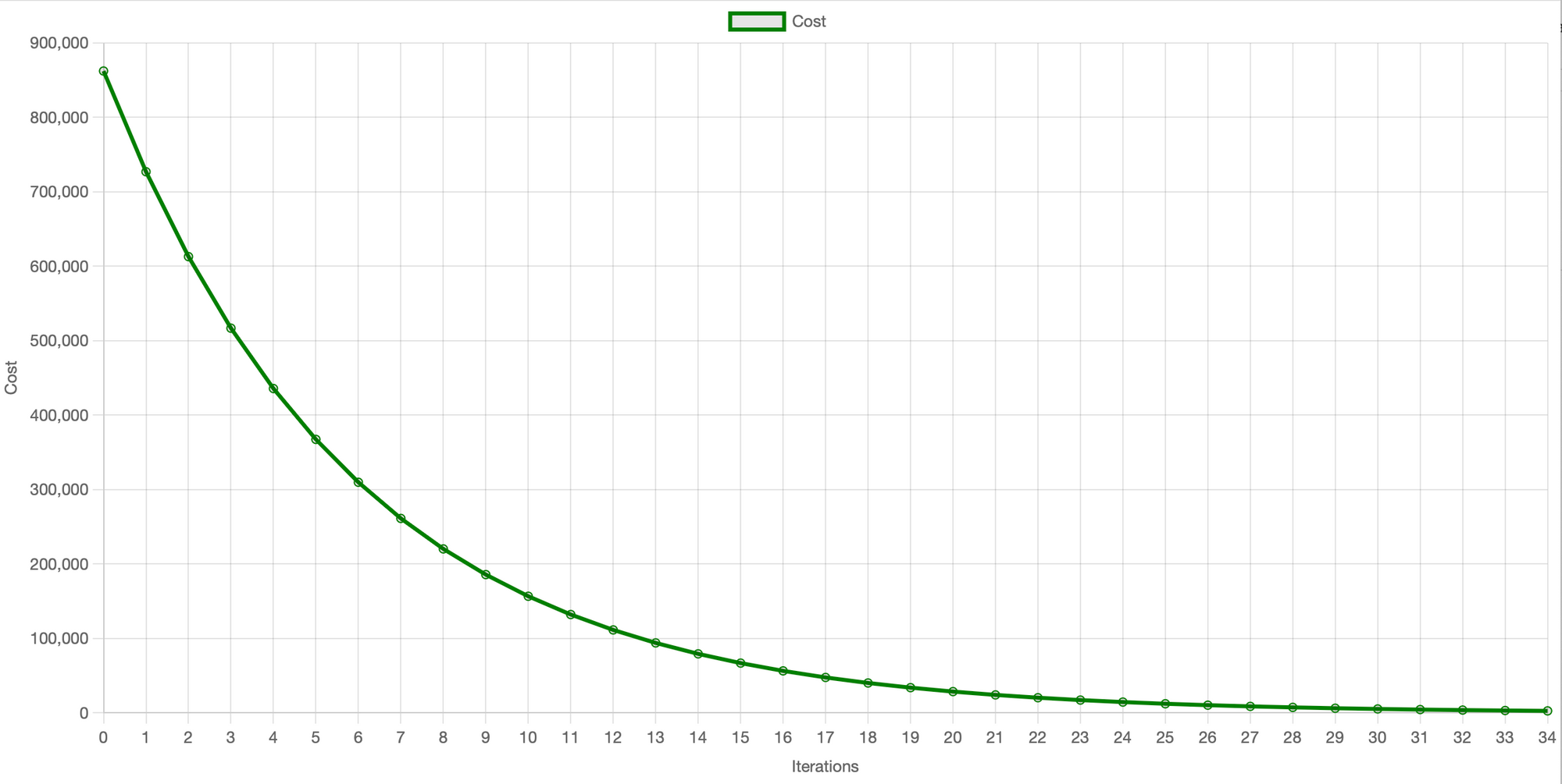
The graph above clearly shows the decrease in cost (MSE) on the y-axis with each iteration. Initially, at iteration 0, the cost is high but each subsequent iteration reduces it as we optimize w and b and re-calculate the cost until it almost reaches the minimum 0 at approximately 35 iterations. This visual representation is referred to as the learning curve. It provides a clear indication of the performance based on the selected learning rate and the number of iterations. Therefore, I highly recommend you plot this graph for your own use case because it can facilitate the determination or adjustment of the learning rate (alpha) and the number of iterations required to achieve convergence.
It's important to note that if your learning rate is too high, the model may never converge. If the learning rate is too low, the model's convergence can be excessively slow, leading to more training time and higher costs. Therefore, finding a good learning rate is important to achieving good results. This process will require some experimentation and fine-tuning.
Conclusion
As we've seen, we covered one of the simplest implementations of gradient descent on a simple linear regression model. There are several other applications to the gradient descent algorithm and it is commonly used in Machine Learning for the purposes of minimizing a given cost function. In future posts, we'll go into other use cases and see how gradient descent is implemented.
As a final note, I'd like to point out that gradient descent is not the best approach when working with linear regression, as there are simpler and more efficient ways of computing the slope (w) and y-intercept (b), as seen in this article.
Thanks for reading and happy coding!